Monday, March 24, 2008

Reverse engineering Google Trends (2): margin of error

As I wrote in my last post, today I'll be quite technical with the margin of error of my computation. And some considerations to try to mimimize this error in the end of my post. Last time on Veronising: I chose a hierarchy of terms which have higher and higher Google Trends curves, to evaluate, by a sequence of rules of three, the frequence of Google searches for the highest term compared to the least looked for.

For the computation I intuitively chose the words such that for each pair of consecutive ones, the first one had a peak approximately twice as high as the second one. The margin of error when reading the value of the curves is approximately 1 pixel, but this absolute error is not the same relative error on the higher, and the lower curve. The higher one always peaks at 113 pixels: 1 pixel of error is less than 1% here. However if the lower one peaks at 50 pixels, it will be a 2% error. If the curve is never over 3 pixels, then the error is more than 30%! So do we have to choose a hierarchy of curves very close to each other? Not necessarily, because in this case we may indeed reduce the error at each step of the computation, but we increase the number of steps (thus, the number of errors) between the least and the most seached.

I couldn't help but mathematically modeling this delicate balance that I've just expressed in a sentence. I call a the ration between the max of the highest and the lower curbe within a pair of consecutive ones (thus a>1). To simplify the problem, I consider that this ratio is constant in my whole scale of words. Then, ideally, I would like to find a word 1 searched x times a day on Google, a word 2 searched ax times, a word 3 searched a2x times... a word n+1 searched anx times.

Now, let's compute the error: instead of reading a height of k pixels for a word, and ak=113 for the next one, say I make an error of 1 pixel, each time too high (this is a pessimistic assumption, actually the error probably alternates, once one reads too high, once too low...). In my computation, without error with the rule of 3 I should find as the number of searches for the highest term:
x.113/k = x.ak/k = xa

The problem is my 1 pixel error, so when I apply the rule of 3 I get in fact:
x.113/(k+1) = x.113/(113/a+1) = x.113a/(113+a)

Thus at each step I multiply by 113a/(113+a) instead of multiplying by a, so for the most searched word, I find x(113a/(113+a))n instead of xan. I underestimate the real value, so to minimize the error I must find the a>1 that maximizes x(113a/(113+a))n.

Second part of the computation: the number of steps, that is n+1 words, of course... but this n depends on a. Indeed we consider that the least searched word (x times) and the most searched one (x'=xan times) are fixed. Then x'=xen ln a, so ln(x'/x)=n ln a and finally n=ln(x'/x)/ln a.

We put this into the upper formula, so we underestimated all the words of the hierarchy, and the highest was evaluated to:
x(113a/(113+a))ln(x'/x)/ln a

which we now have to maximize according to a. A quick analysis of this function at its limits shows that it tends to 0 in 1+, and to 1 in +∞. Very well, it expresses the dilemma I was mentioning in the 2nd paragraph. However it doesn't give us where the max is reached, and neither Ahmed the Pysicist, nor Julian the Mathématician, helped respectively with Mathematica and Maple, could give me a nice formula, there are still some ugly RootOf(...) in the formula.

No problem, we'll just find an approximation using Open Office Spreadsheet. The file is there, and here is the curve obtained for a ration of 20,000 between the most searched and the least searched word (the figure approximately corresponds to what I found for my hierarchy):
So the minimal error is reached for a approximately equal to 2.75 (i.e. a maximal height of 41 pixels for the lower curve). Then it's less than 25%. Of course it seems a lot, but remember the remark on how pessimistic this scenario was, with errors cumulating by successive underestimations. I still have this interesting theoretical question: is it possible to compute the expectancy of the error on the computed value of the most searched word, if at each step the error randomly varies between -1 and +1 pixel? ?

One can also notice the curve increases a bit faster on the left than on the right. As shown in green on the graph, it seems that we'd better choose a hierarchy such that consecutive reference words have a number of searches ratio of 4 rather than a ration of 2.

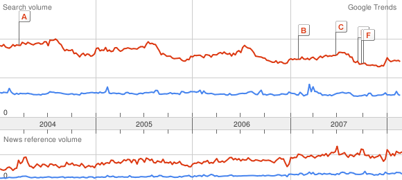
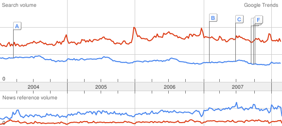
Now, here are some other hints to improve the accuracy of the computation. First, measure accuracy: instead of just measuring the maximum, where we know there is an inevitable error, we can try to compute it from measures with less errors. I come back to my example from the previous post with cat, dog, and phone:
Comparison cat ~ dog (curve 1) : 65 px ~ 113 px
Comparison dog ~ phone (curve 2) : 69 px ~ 113 px

Except that instead of measuring the maximum of dog, we can evaluate it the following way: do the average of the values of the curve 1 for dog, the average of the values of the curve 2 for dog. Then deduce a very accurate scale change. Finally multiply the maximum of dog on the curve 1 (that is exactly 113 pixels, no error here) by this scale change!

Another problem now: how to obtain the average of the values of a Google Trends curve? With the CaptuCourbe, of course! Be careful here: some values may not be retrieved by the CaptuCourbe (color problem, for example the curve is cut by a vertical black line hanging from a Google News label bubble). So you have to compute the average of the curves on values you really managed to retrieve!

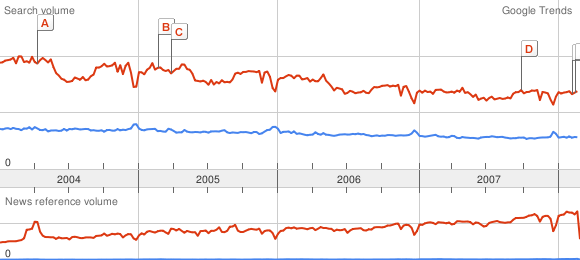
One more thing, the CaptuCourbe is not very accurate because it gets the values of all pixels of some color from a curve, and computes the average, for each column of retrieved values. I've developed a new version, online soon, which allows to get the maximum of the heights of pixels of some color. I'm using this functionality in my method to compute the max, however it's still the average choice I make to get the average of the curves. This is not a small detail, as you can see on the Britney Spears Google Trends curve, that I extracted in both ways:
A 20% error in the measure of many peaks using the pixels of the same color is really something!

So, to close this series of posts on the vertical scale of Google Trends, I still have some questions left. First, get a "value of the foo" in the number of daily searches. Then I could try to program the whole chain of curve retrieval, measures, and computations, as described in my first post, to provide a utility which would add the vertical scale to a Google Trends curve. Anyway don't expect too much, I'd better wait and see whether the API Google is preparing will provide this data.

Estimating the number of searches for some keyword is still a nice challenge., I've discovered GTrends Made Easy, a freeware which gives some estimations computed with a method similar to mine here (in fact he does only 1 rule of three, comparing the request word with a reference word for which he knows the number of Google searches, approx 500 ; that is words which appear between 5 and 50000 times a day, that is less than 100 foo), which was described on this YouTube video.


This post was originally published in French: Rétroingéniérie de Google Trends (2) : marge d'erreur.

Monday, March 10, 2008

Reverse engineering Google Trends (1)

Last December I started to create a simple program to retrieve the values of a curve from a picture the CaptuCourbe, which is still not translated in English, but has an English tutorial. One of the possible use of this free software is retrieving and comparing Google Trends curves. Except Google Trends curves have a major problem: the vertical scale is not hidden! On top of that there is no zooming tool, so we can't directly compare curves of drastically different heights. The maximum height of a curve is always 113 pixels, so you won't be able to know if a word has been searched 1000 or 10.000 more than another.

Here is a hierarchy of English words, in a decreasing order considering their Google searches according to Google Trends : of, free, sex, car, dog, gun, muscle, knife, torn, filming, separating, fooling.

They can be used to create a scale for Google Trends. It may not be very accurate, but would still be useful to get quantitative values. To compute it, I google-trended pairs of successive words in the hierarchy above. This gives me the scale change for each pair, by measuring the height (in pixels) of the maximum of each curve. Here is a picture to explain what I mean:

As I do that for successive words, I get values like this:
Comparison cat ~ dog : 65 px ~ 113 px
Comparison dog ~ phone : 69 px ~ 113 px
thus I can deduce by a subtle use of the rule of three:
cat ~ dog ~ phone : 65 ~ 113 ~ 113*113/69=185,06
considering the scale of the first line or:
cat ~ dog ~ phone : 69*65/113=39,69 ~ 69 ~ 113
with the scale of the second one.

I did this computation for all 11 words to get the following maximum values, where I defined the reference as the maximum of fooling. Of course, I call this new unit the foo:
Be careful, what you have to remember is not only those different values, but also the position of the maximum which reaches those values, that's why each word above links to a picture of the curve to localize its maximum value. Indeed if you want to determine the value of a peak for a new word, either you understood this rule of three principle and then you can have fun computing it directly, or you just use the CaptuCourbe, with the reference curve whose max is just above the peak you want to compute:
For example here about 800 foo for Manaudou in December 2007, to compare with the 240 foo of the Bruni peak, the 470 foo reached by Obama, the 1000 foo of Britney the 3200 foo of the tsunami de 2004 and the 5700 foo of... Janet Jackson after Superbowl 2004!

Now, let's get to the bad news:
- the error propagated by applying 10 times the rule of three will be the topic of my next post, quite technical (there will even be a pretty nice equation that neither Maple nor Mathematica can simplify)... just consider that the numbers above must be accurate +/- 10%.
- the Google Trends curves vary a lot (maybe it's just a discretization problem, but in this case it's quite strange that the Google News discretization below is the same), as you can see on this animated gif (created with the great and simple UnFreez) :
So be careful if you use one of those reference words: you have to remember the value of the peak, its position, but you may also want to superimpose the reference curve that I linked to the word, to check that the reference curve in the picture you're using has its max at the same place, and has the same scale. Try to correct it if it's not the case.
- the scale remains relative, to get an absolute one the question would be: how many Google requests is 1 foo? After my post in French, I got some pretty good comments on this idea, I sum them up here. First we have to be careful that the curves don't show the number of searches, but just the proportion of searches for a word among all searches in some period of time. This would explain why the Janet Jackson buzz was so high, it's difficult to compare the number of searches corresponding to 5700 foo in 2004 to 800 foo today. Anyway it's still possible to get an idea of the proportion from the number of searches, by trying to find data on the evolution of the number of Google searches in the past years, this must exist on the web (Alexa, at least...). Let's be more accurate about these values: on the 2004-2008 pictures, as I said I have no idea how the discretization is made, however on the yearly or monthly pictures, it's quite clear that we find, respectively, the weekly and the daily numbers. So what I'm looking for right now is, for some word, the number of searches it corresponds to. Elandrael had the brilliant idea of using Google Adwords stats, to get at least a lower bound on this number. For the moment I only got one Google Adword to apply this idea, which would show that a one foo peak corresponds to more than 20000 searches in a month, that is more than 4000 searches if we look at the weekly value in a yearly curve. So of course I would love to get some other statistics like this to confront the data, just contact me privately if you don't want to write on this blog the Adword you're paying for and its stats. On the same principle, you can also contact me if you have the stats for a common word in which your website appears as the first Google Answer.


This post was originally published in French: Rétroingéniérie de Google Trends.

Source files: the Google Trends curves of each word are linked above, here is the spreadsheet file that I used to compute the values in foo (it's quite a mess though, more details to understand it in my next post).

Sunday, March 2, 2008

The birth of a buzz, live

I've been dreaming for some time to follow on the web the birth of a buzz, and evaluate the reaction of the tools dedicated to their analysis and detection. I would have prefered better circumstances, but I was able to do it for the tragedy of the Northern Illinois University shooting two weeks ago.

The name of the gunman was not published on the evening of the drama. But 10 hours later, the Chicago Tribune provided
enough elements to guess it on their website
. Of course they wrote quite hypocritically:
The Tribune is not naming the gunman because police have not officially completed the identification of his body.
A simple search for articles co-signed by Jim Thomas with the keywords "self-injury" and "prison" would identify the suspect: Steve Kazmierczak. At 8:10GMT, a visitor of the Wikipedia modifies the article about the shooting to add that name. 30 minutes later, a first blog post cites it, its author updates it many times to add other info found on the net. The name appears then in a live journal and on a forum, and at 10:33 is cited by the Daily Mail (the article has been update since). Then people start to google it a lot, and it reaches the top of the "hot trends" list. It's then cited by some splogs, which apparently make money by citing those trends sometimes with extracts of web pages about it, retrieved automatically. At 14:42, the Associated Press announces that the police gave the name: Steven Kazmierczak. I stopped following the buzz there, as articles or webpages about it then used "Steve", "Steven" or "Stephen".

Anyway, following the first hours gave me the opportunity to see how fast the web reacted. As I mentioned it, the Wikipedia first gave the name. Once more we can wonder about the ethics of the project, and note that it has become THE place to find the latest scoops. See how reactive it is to the death of a celebrity? You can even use the Wikirage tool, which put on top of its hot article list on February 13: Henri Salvador, Imad Mougniyah, et Badri Patarkatsishvili.

About the blogosphere tools, one can notice that BlogPulse isn't very responsive. Of course Google Blogsearch detects quite fast the first blogpost on the topic, in a Blogpost blog... However Blogsearch and Technorati seem to have a similar efficiency: the Technorati curve is a bit higher after 2PM because of some splogs, which Google Blogsearch didn't display (on purpose, i.e. better splog detection?).

The reaction of search engines on the "Steve Kazmierczak" request is also quite interesting. They don't detect the buzz in the first hours, except Google. Even if it's not very clear on the graph, the number of relevant results increases from 61 at 10:30 to 68 at 4PM (and those new pages deal indeed with the gunman). But this contrasts with the big rise of the total number of results, which reinforces the mystery on Google numbers. Did the number of pages for this request really double in 5 hours, or is it just a suspicious approximation?

But the most important may be in the Google Trends curves. Before the press dared to give the gunman's name, before Wikipedia learned of it, before the tabloids found out, Google knew, with the first searches on the name less than 3 hours after the shooting. Their leadership over other search engines also gives them a direct access to information, and their tools are ready to treat this as much as they can. With geolocation in particular, to determine the origin of requests, and maybe identify a local buzz. So when will Google launch a press agency or a tabloid, to uncover scoops and rumors hours before the Daily Mail? And who can access those Google Trends data live today? On the website, the curves are currently updated after 48 hours, not available for words not searched enough, the horizontal scale is not explained (I'm guessing that the 4AM dot represents the number of searches from 3AM to 4AM but I may be wrong), without even mentioning the lack of a vertical scale! A Google Trends API may give the possibility to access this data, and give back to the internauts the knowledge learned from them.


This post was originally published in French: Suivi en direct de la naissance d'un buzz.
The data I gathered and used for the graphs (OpenOffice Spreadsheet file)